Andrew H Beck, Cheng-Han Lee, Daniela M Witten, Briana C Gleason, Badreddin Edris, Inigo Espinosa, Shirley Zhu, Rui Li, Kelli D Montgomery, Robert J Marinelli, Robert Tibshirani, Trevor Hastie, David M Jablons, Brian P Rubin, Christopher D Fletcher, Robert B West, Matt van de Rijn
| Home |
| Home |
| LMS Images |
| Histological Images |
| Figures |
| Figures |
| WebPortal |
| Stanford Tissue Microarray Consortium Web Portal |
| Authors |
| Authors |
Figures (click on figure to view full size) | |
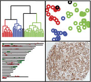
Figure 1. Unsupervised clustering of 51 LMS samples reveals 3 reproducible molecular subtypes.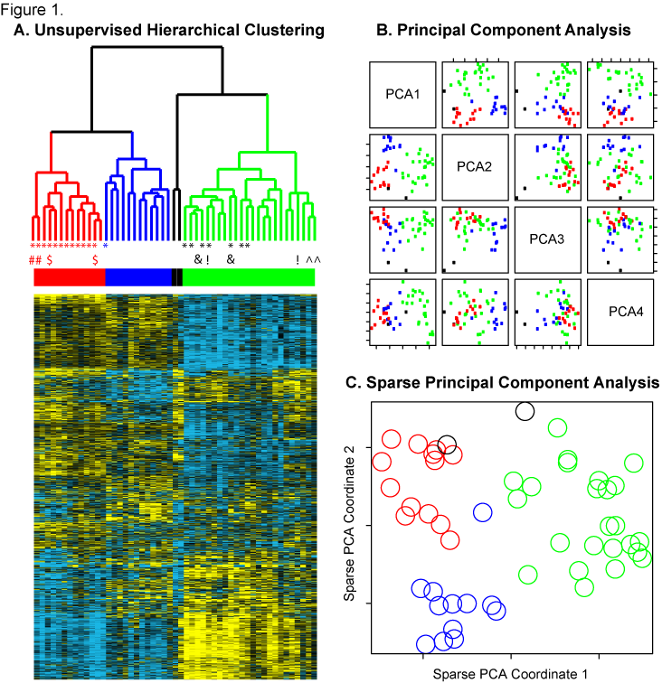 A) Unsupervised hierarchical clustering was performed on 51 LMS samples with 3038 genes that showed at least 1 standard deviation across the samples. The 20 samples that were also profiled for DNA copy number changes with aCGH are indicated by an asterisk. The 5 paired primary-metastasis samples are indicated by a paired symbol (#,$,&,!,^). On the sample dendrogram, the Group I cases are heighted in red, Group II blue, and Group III green. The 2 cases that did not cluster into a group are indicated in black. Within the heatmap, yellow indicates relatively increased expression, black indicates median expression, and blue indicates relatively decreased expression. B) Principal Component Analysis of the 51 LMS samples with 3038 genes. Each sample is represented in the figure by a colored box. The color indicates the clustering designation made by hierarchical clustering: red = Group I, blue = Group II, and Green = Group III. Most of the variance between the 3 groups is captured in the first two principal components. C) Sparse Principal Component Analysis. The 51 LMS samples were plotted against the sparse PCA coordinate 1 (containing 45 genes) and sparse PCA coordinate 2 (containing 40 genes). Each sample is represented by a colored circle, and the color indicates the clustering designation made by hierarchical clustering: red = Group I, blue = Group II, green = Group III. Most of the variance between the 3 LMS molecular subtypes is explained by these 2 sparse principal components. Figure 2. Array Comparative Genomic Hybridization of 20 Leiomyosarcoma Samples.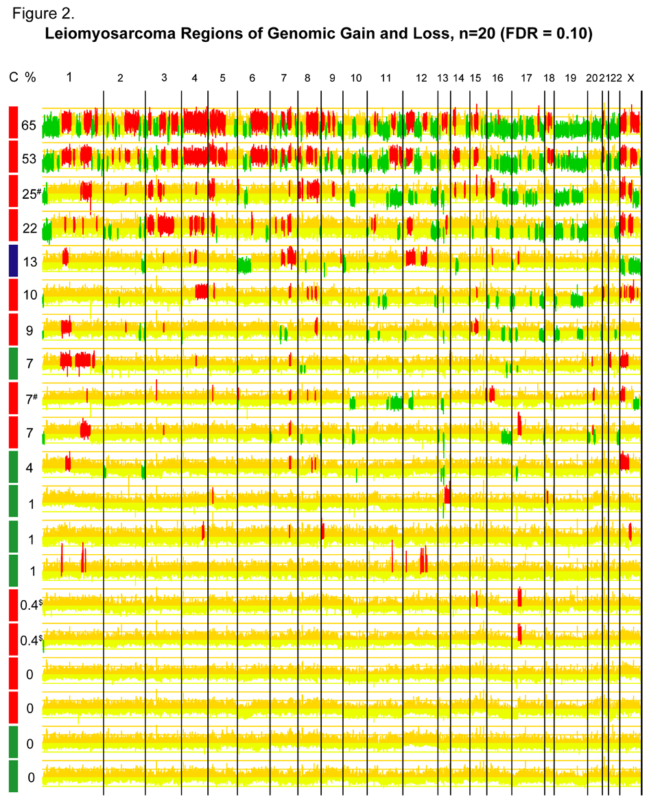 The 20 samples are arranged along the y axis and ordered according to amount of DNA copy number changes. Chromosomal locations are indicated along the x axis. Copy number changes were called using the cghFLasso algorithm with an overall false discovery rate of 0.10. Regions of genomic gain are indicated in red and loss in green. The proportion of genome showing gain or loss is indicated to the left of each row. The gene-expression defined molecular subtype is indicated on the colorbar on the left: red = Group I, blue = Group II, green = Group III. The Group I cases show significantly increased regions of genomic gain/loss compared to the Group III cases (p=0.04). Figure 3. Protein Expression of Group I Markers on Leiomyosarcoma Tissue Microarray.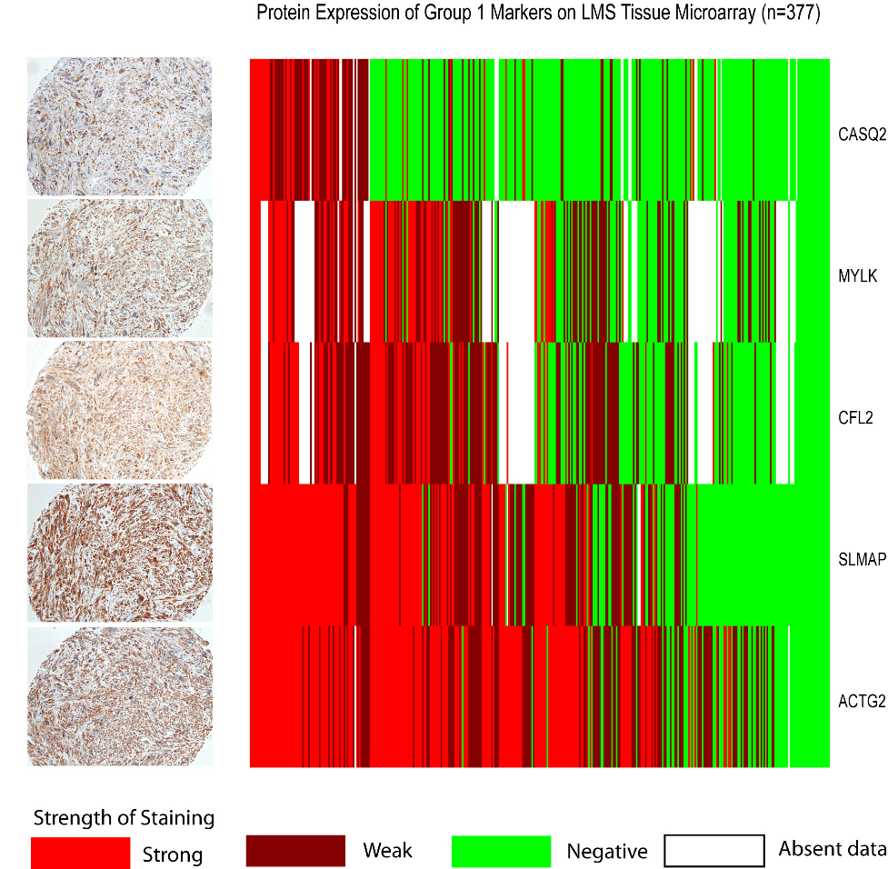 We performed IHC for 5 markers that showed high levels of expression in Group I LMS in the gene expression analysis (CASQ2, MYLK, CFL2, SLMAP, ACTG2). The LMS TMAs contained a total of 377 samples that were scored as strong positive (bright red in the heatmap), weak positive (dull red), or negative (green). The antibodies are listed along the y axis and the 377 samples along the x axis. Missing data is indicated by white in the heatmap. Pictures of an LMS sample showing strong expression of all 5 stains is shown to the left of the heatmap (magnification=200x). The five stains showed significantly correlated expression (all pairwise Spearman's rho p < 0.005, with a minimum correlation of 0.17 between ACTG2 and CASQ2 and a maximum correlation of 0.66 between ACTG2 and SLMAP). Table 1. Multivariate Cox Regression Analysis of Disease Specific Survival from LMS Tissue Microarray (n=124).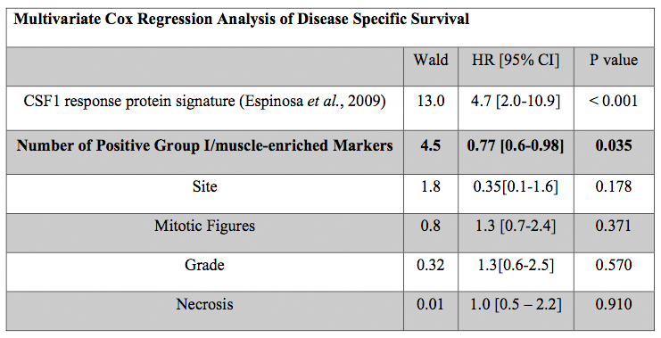 In the multivariate model, only the CSF1-response protein expression signature and the expression of Group-I/muscle-associated proteins showed a significant association with survival. In the table, the first column lists each variable included in the model, the second column lists the variable's Wald test statistic, the third column lists the variable's hazard ratio (HR) and 95% confidence interval (CI), and the fourth column lists the variable's Wald test p value. Figure S1 - Correlation of 51 LMS samples with LMS Group Centroids.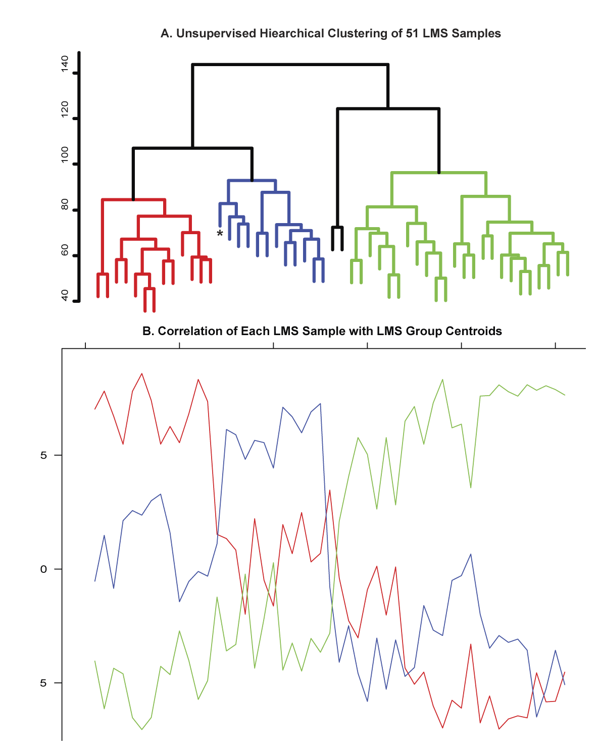 A. Unsupervised hierarchical clustering was used to divide the LMS cases into 3 predominant groups. The dendrogram leaves are labeled red for Group I cases, blue for Group II cases, green for Group III cases, and black for the two cases that did not fall into 1 of the 3 predominant LMS clusters. B. A centroid was created for each LMS cluster, and the Pearson correlation between each LMS sample and the 3 centroids was determined. The LMS samples are ordered along the x axis according to the unsupervised hierarchical clustering in A. The correlation of each sample with the LMS group centroids is plotted along the y axis: correlation with the Group 1 centroid is indicated by the red line; with the Group II centroid by the blue line, and with the Group III centroid by the green line. The horizontal line underneath the plot is color-coded according to the samples' group designation by hierarchical clustering (red=Group I, blue=Group II, green=Group III, black = no group). This figure demonstrates that all but 1 of the 49 LMS samples that fell into Groups I, II, or III by hierarchical clustering shows the highest correlation with its group's centroid. There is 1 Group II case that shows relatively similar correlation with the Group I and Group II centroids, but clustered into Group I by the hierarchical clustering. This case is indicated by an asterisk on the dendrogram tree in A and below the horizontal color bar in B. Neither of the 2 outlier cases by unsupervised hierarchical clustering shows strong correlation with any of the LMS group centroids. Figure S2 - Clustering of 51 LMS samples with a diverse set of soft tissue tumors (n=291, spanning 25 diagnostic subtypes).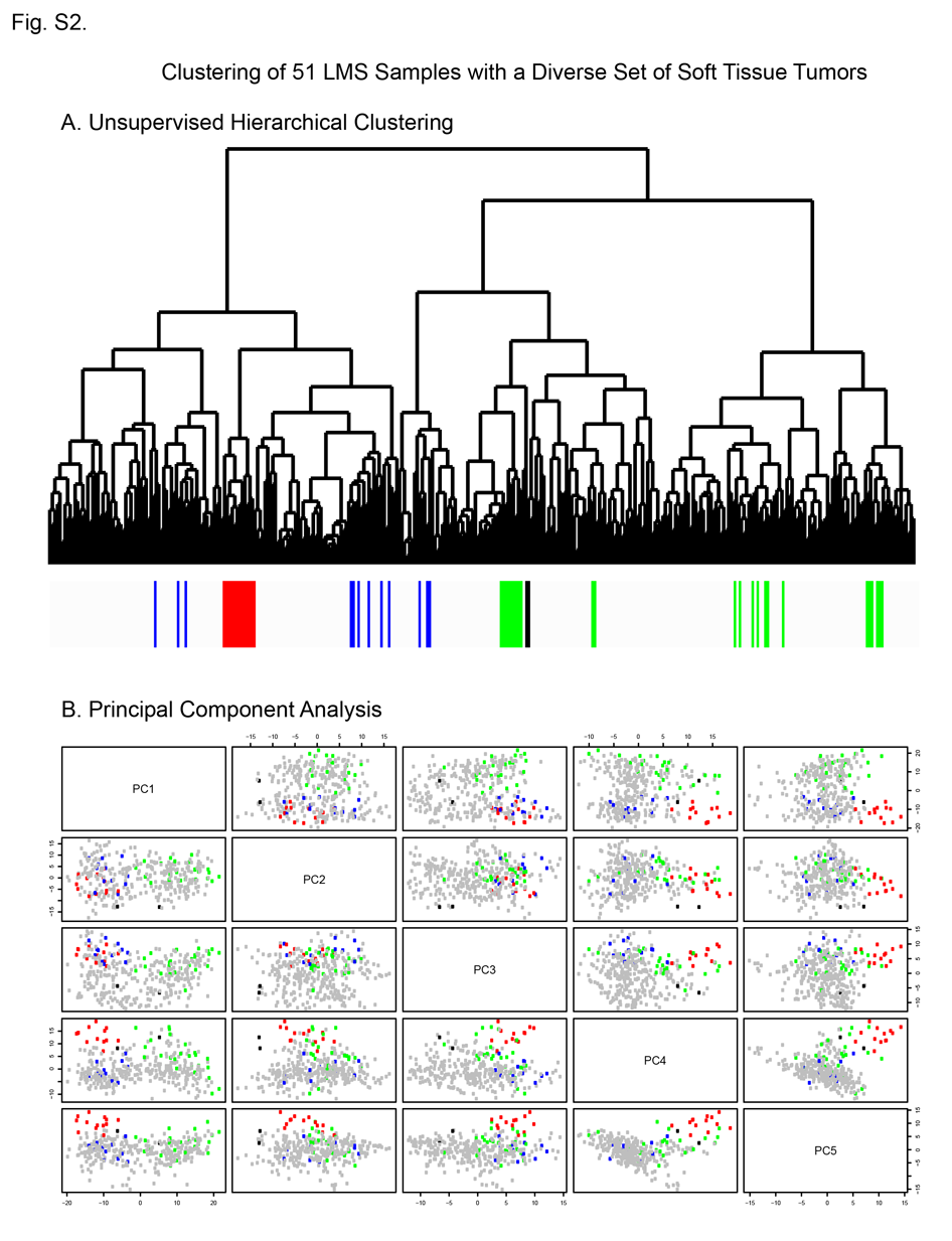 A) Unsupervised hierarchical clustering sample dendrogram shows that the 12 Group I cases cluster tightly together, while cases from the other LMS subtypes are intermixed with other soft tissue tumors. B) Principal Component Analysis. Each sample is indicated by a colored dot: the non-LMS cases are grey, the Group I LMS samples are red, Group II LMS samples are blue, and the Group III LMS samples are green. This analysis shows that the separation of the Group I cases from the other LMS and STTs is explained primarily by the 4th and 5th principal components. The other LMS subgroups remain intermixed with the other STTs. Figure S3 - Unsupervised Hierarchical Clustering of GSE2553 Data Set With Genes Highly Expressed in LMS Subtypes.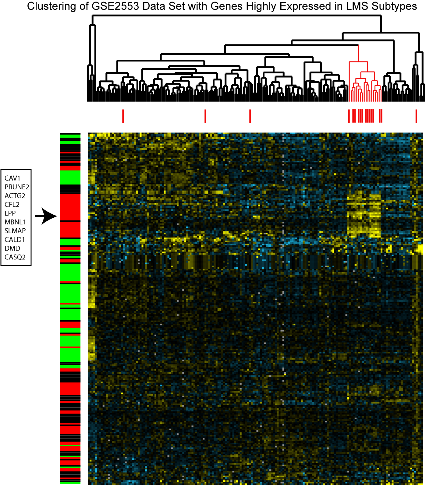 The GSE2553 contains gene expression data from 181 sarcomas, including 17 LMS samples. The samples are clustered along the x axis, and the 17 LMS samples are labeled with a red bar. The sarcomas are clustered with genes highly differentially expressed in each LMS subtype. The colorbar to the left of the heatmap indicates whether that row's gene was highly expressed in LMS group I (red), group II (blue), or group III (green). Within the heatmap, yellow indicates relatively increased expression, black median expression, and blue relatively decreased expression. This analysis shows that most of the LMS (13/17) cluster together and show high levels of expression of a core set of genes highly expressed in Group I LMS, including: CAV1, PRUNE2, ACTG2, CFL2, LPP, MBNL1, SLMAP, CALD1, DMD, and CASQ2. A clusterRepro analysis was performed and showed significant reproducibility of only the Group I LMS in this dataset. Figure S4 - PAM-FL aCGH Centroid for Group I LMS.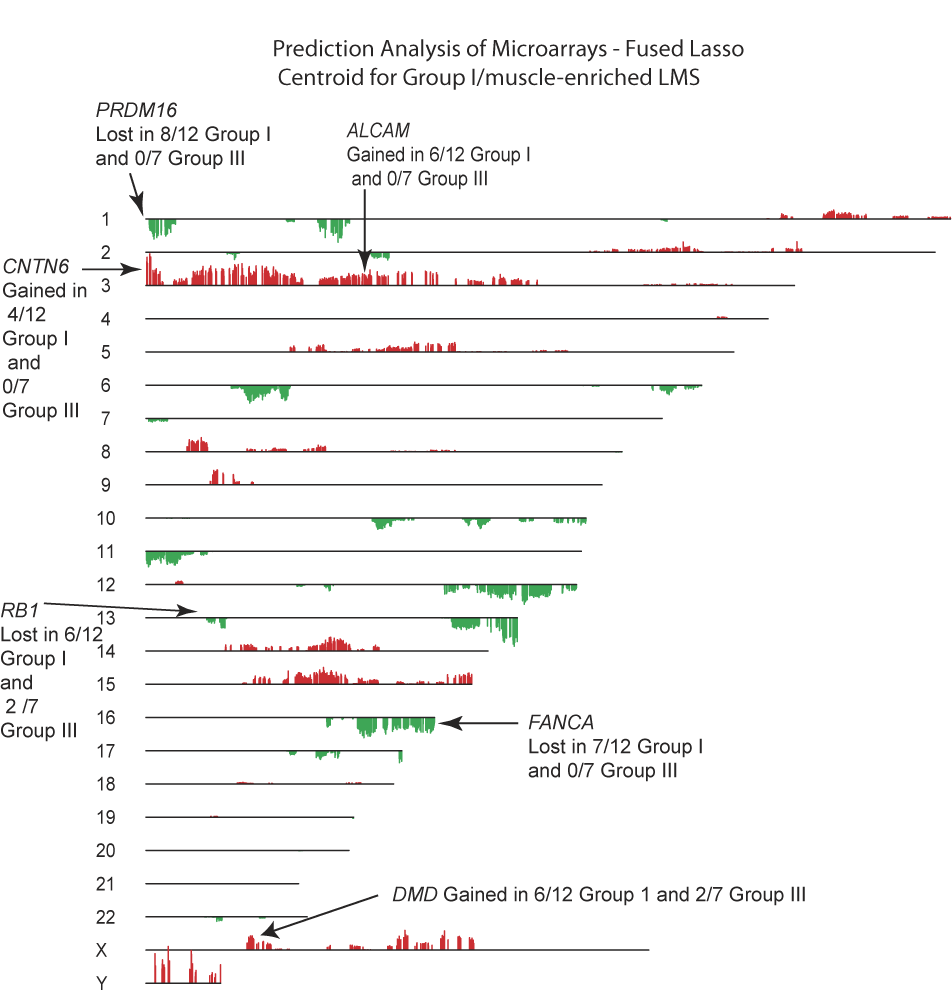 The Group I LMS aCGH centroid is a display of the genomic changes that best characterize LMS Group I relative to LMS Group III. Several candidate genes from regions of genomic gain or loss are displayed. Figure S5 - Unsupervised hierarchical clustering of the 51 LMS samples with ~13,000 genes.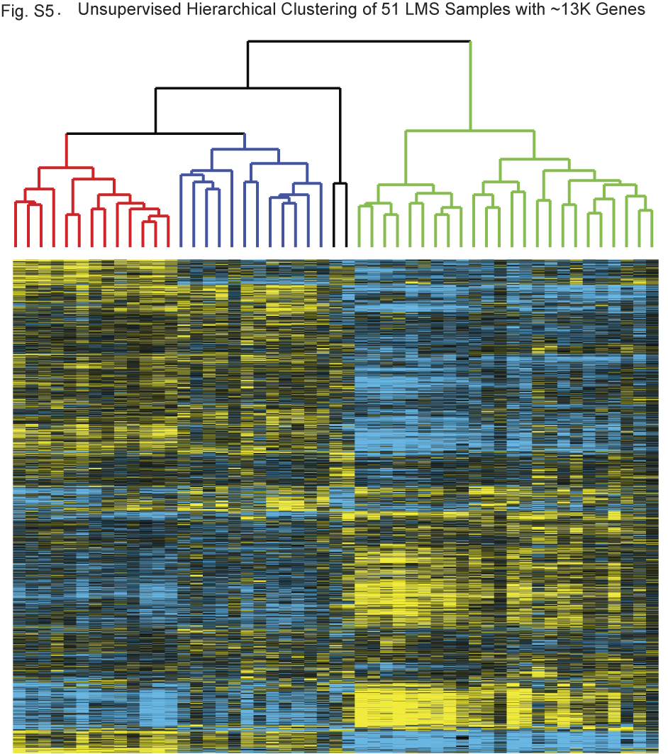 To ensure that the stringency of our gene filtering technique did not significantly alter our clustering results, we performed clustering with a less stringent filtering criteria requiring each gene to have 70% data and present and show at least 0.5 SD of variation across the samples. The samples clustered into identical subgroups as observed in the primary analysis (based on ~3K genes). |